Quantum
Mechanics

Our interest is in the x-dependent equation (i.e. the part that is independent of time). The equation in x is:

¹/_ψ(x) ^d2ψ(x)/_dx² = -β²

and hence we get

^d2ψ(x)/_dx² + &beta²ψ(x) = 0

This is a time-independent classical wave equation. It is easy to solve, because all we have to do is take the β²sinψ(x) back over to the right hand side and then look for a function that, when we differentiate it twice, we get the same function again times -β². One solution would be sinβx, and another (remember Euler again) would be e^βi...

The solution ψ(x) = Asinβx is equivalent to the time-dependent solution in Exercise 3.5 if we set t = 0 (check this for yourself). Hence we can identify β with 2π/λ, and we can then rewrite the time-independent wave equation in the form:

^d2ψ(x)/_dx² + 4π²/_λ² &psi(x) = 0(13.17)

This differential equation is in precisely the same form as the key equation for quantum mechanics, the Schrödinger wave equation, and in fact we will use it to (sort of kind of) derive the Schrödinger wave equation. The quantum treatment of any chemical problem begins by setting up appropriate boundary conditions for this wave equation. The solutions ψ(x) of the wave equation are known as wavefunctions: they contain all the information we can hope to learn about the problem. That information can be retrieved by performing certain mathematical operations on the wavefunction. These three steps:

1. setting up the wave equation;
2. solving it to obtain the wavefunction;
3. using the wavefunction to obtain energies, momenta, etc...

are standard procedures for any quantum mechanical problem.

The Schrödinger equation

This section of the text derives Schrödinger's equation by assuming that atomic and molecular particles obey the time-independent wave equation, and that the wavelength of the particles obeys the de Broglie equation, λ = h/p.

Recall that we can write the total energy, E, as a sum of kinetic and potential terms:

Using p² = (mv)² = 2mK = 2m(E - V), we obtain p = [2m(E - V)]½, so that using the de Broglie relation λ = hp yields

λ² = ^h2/2m(E - V)

Substituting this into the time-independent wave equation (13.17) we get

^d2ψ(x)/_dx² + 4π²2m(E - V)/_h² ψ(x) = 0

which is readily rearranged to obtain the Schrödinger equation for a particle of mass m moving in one dimension with energy E:

^-h2/8&pi²m ^d2ψ(x)/_dx² + Vψ(x) = Eψ(x)

The Schrödinger equation can be rewritten in a more compact form:

H²/2m ^d2ψ/_dx² + Vψ = Eψ(13.20)

where H = h/2π (pronounced “h-bar”) and V and ψ are both functions of x. The first term in this expression can be identified with the kinetic energy of the system, and it has a similar form for all systems. But the potential energy term depends greatly on the system; for a free particle V = 0, and for a harmonic oscillator V = ½kx²

An interesting insight into the relationship between the form of the wavefunction ψ and the kinetic energy K can be obtained from

λ = ^h/₍2m(E - V))^½

= ^h/₍2mK)^½

Hence the greater the kinetic energy K, the smaller the wavelength. But we can relate the second derivative d²ψ/dx² to the curvature of the wavefunction (i.e. the rate of change of slope). When a wavefunction is sharply curved (has lots of squiggles) the kinetic energy is large. When ψ is not so sharply curved (long wavelength, few squiggles) K is small. The association of curvature with kinetic energy is often a valuable clue to the interpretation of wavefunctions.

Operators and observables

The Schrödinger equation can be rewritten in the more succinct form

(Ĥψ = Eψ)

(13.29)

where Ĥ is now an operator, something that operates on the wavefunction ψ(x). In this case we have

Ĥ = ^{- η2}/2m ^d2/_dx² + V

or in words, stepwise, take the second derivative of ψ, multiply it by H²/2m, and add to it the product of ψ. The operator Ĥ  is a special one in quantum chemistry and is called the Hamiltonian operator.

The Schrödinger equation Ĥψ = Eψ is what is known as an eigenvalue equation:

(operator) × (function) = (constant) × (function).

Symbolically, these special equations are of the form

Ôf = ωf

where Ô is the operator, ω is the eigenvalue of the operator Ô (e.g. E is the eigenvalue for Ĥ) and f is the eigenfunction corresponding to that eigenvalue. As another example, e^ax2 is an eigenfunction of d/dx, but e^ax2 is not an eigenfunction of d/dx.

Eigenvalue equations are important in quantum mechanics because they are repeated for many other properties apart from energy, properties that in quantum mechanics are called observables. In general we can write

(operator) × (wavefunction) = (observable) × (wavefunction).

Therefore if we know the wavefunction and operator we can predict the outcome of an observation of that property by picking out the factor ω (the eigenvalue) in the eigenvalue equation.

Table 14.1, p. 313 of E&R, gives a convenient summary of operators for various observables (such as position, momentum, energy), along with their classical counterparts.

Properties of the wavefunction

One of the basic assumptions in quantum mechanics is that the state of a system (e.g. an electron, proton, atom, molecule….) can be described by its wavefunction, in just the same way that the displacement of a macroscopic string can be described by the wavefunction ψ(x,t).. Moreover, the wavefunction contains all the information we need to know about the system! And just as in classical mechanics, not just any old mathematical function will do – it must satisfy certain constraints in order to be physically reasonable.

The mathematical constraints include:

• ψ(x) and dψ(x) / dx must be everywhere finite;
• ψ(x) and dψ(x) / dx must be single-valued everywhere;
• &psi(x) and dψ(x) / dx must be continuous everywhere.

Some examples of acceptable and unacceptable wavefunctions are given in Fig. 14.2, p. 312 of E&R. It is always advisable to keep these requirements in mind when seeking solutions to the Schrödinger equation: they are the key to physically correct solutions.

The Born interpretation of the wavefunction

Assume that we can solve for ψ for a particular problem. What does it mean? In what ways can we learn about the properties of the particular system, be it the H atom, water molecule or a complex organic dye?

The answer to these questions, suggested by Max Born in 1926, showed that a wavefunction gives a description of a particle in terms of probabilities. Specifically, for a one-dimensional system, the probability of finding the particle in the region of space from x to x + dx is given by ψ²(x)dx (often this is written allowing for the complex nature of ψ - for example ψ(x) = Ae^2x - as a product of ψ and its complex conjugate ψ^*).

Thus ψ² is a probability density (density, since it must be multiplied by infinitesimal length dx to get a probability), and ψ itself is called a probability amplitude.

We can then write down the probability of finding a particle (described by the real wavefunction ψ(x)) in a particular region of space, say between x = a and x = b, a < b,

P(a ≤ x ≤ b) = ∫_a^b&psi²(x)dx

i.e. the sum over all infinitesimal probabilities P(x)dx over the region.

Born's interpretation imposes very important constraints on the nature of the wavefunction, and it should now be clear why wavefunctions must be bounded (i.e. not reach infinity), single-valued, and continuous. A very important condition on a physically meaningful wavefunction is that of normalisation. Clearly, if we extend the limits of integration to (in words, over all space), the integral must equal unity: the particle must exist somewhere!

∫_-∞^∞ψ²(x)dx = 1(14.2)

Wavefunctions obtained from the Schrödinger equation will always have a multiplicative constant, N, the normalisation constant.

The expectation value

This section of the text introduces the operators that are the quantum mechanical analogue of a collection of properties of the system, or observables, that are familiar to us from classical mechanics. There are two things we might want to do with these operators: find the result of an individual measurement, and find the average value we would obtain, if we carried out a large number of measurements. More often, we want to find the average value, since the general eigenvalue equation Ôf = ωf will have an infinite number of solutions ω.

In quantum mechanics the average value of an observable A whose operator is  is called the expectation value and is written like so:

<A>

It is calculated from

<A> = ^{∫ ψ ψdτ}/_{∫ ψ²dτ}

(14.4)

where dτ indicates integration over the appropriate variable(s). If the wavefunction ψ is normalised, than the bottom term of the expression is clearly equal to 1. The meaning of the integrand is that ψ is operated on by  to give a new function, and then this function is multiplied by ψ. It follows from this expression that, in the special case of the wavefunction ψ being an eigenfunction of the observable A with eigenvalue a:

<A> = a.

Translational motion: the particle in a box

Unfortunately, there are only a few systems for which solutions of the Schrödinger equation are straightforward and analytic (i.e. have a convenient mathematical form giving an equation that can actually be solved). These systems include (in order of increasing complexity): the free particle, the particle in a box, the harmonic oscillator, the rigid rotor, and the hydrogen atom. We will investigate each of these in turn.

The Schrödinger equation for free translational motion in one dimension is

^-H2/_2m ^d2ψ/_dx² = Eψ(i.e. V = 0)

It is easily shown that general solutions to this equation are of the form

ψ = Acoskx + Bsinkx

All values of k are permitted, hence all energies are allowed.

We are now ready to consider the problem of a particle in a one-dimensional box: a particle of mass m confined between two walls at x = 0 and x = a (see Fig. 15.1 p. 321 E&R). The potential energy is zero inside the box but rises abruptly to infinity at the walls. The Schrödinger equation for the region between the walls (where V = 0) is just that for a free particle, so the general solutions are the same as for a free particle.

Because the particle is restricted to the region (0, a) the probability that the particle is found outside this region is precisely zero. Hence ψ(x) = 0 for x outside (0, a). Mathematically, this is how we restrict the particle to the confines of the box. But to be an acceptable solution ψ(x) must be continuous and therefore ψ(0) = ψ(a) = 0, since any other choice would yield a discontinuity at the walls of the box. These are two boundary conditions on the wavefunction, which have dramatic implications for the form of the solution.

Using ψ(0) = 0 we must conclude that A = 0, since sin0 = 0, cos0 = 1. Hence our most general wavefunction must be of the form:

ψ(x) = B sin kx

But the amplitude at the other wall must also be zero, hence

ψ(a) = B sin ka = 0

This can have two solutions: either B = 0 (implying ψ = 0 for all x, a true but useless solution- such solutions are called trivial) or k must be chosen such that sin ka = 0 latter condition is satisfied provided

ka = nπ,n = 1, 2, 3, ...

Also, since k and E are related, we obtain

E = ^k2H2/2m = ^(nπ/a)2H2/2m = ^n2h2/8ma²,n = 1,2,3,...(15.17)

You should recognise immediately that the energy of a particle in a box is quantised – it can only take on certain values - and that this quantisation arises directly from the boundary conditions that ψ must satisfy to make it an acceptable wavefunction. The integer n is known as a quantum number. We can impose normalisation on the solutions to solve for the amplitude, B:

1 = ∫_-∞^∞ &psi²dx

= B²∫₀^a sin² kxdx

= B²½∫₀^a (1 - cos2kx) dx

= ½B²[x - 1/_2k sin 2kx]₀^a

= ½B²[a - 1/_2k sin2ka - 0 + ¹/_2ksin 2k0]

= ½B²a

∴ B = √²/_a

From this we can see that the wavefunctions are of the form:

ψ_n(x) = √²/_a sin^nπx/_a,n = 1,2,3,...(15.15)

where we have labeled the wavefunctions with the quantum number n.

The wavefunctions are the same as standing waves set up in a vibrating string; the energy increases with the number of nodes.

(The energy levels can also be derived independently by observing that the wavelength is directly related to the size of the box via a = nλ / 2 (i.e. an integral number of half wavelengths)) and using this information in the de Broglie relation).

Several properties of the particle-on-a-box solutions yield considerable insight. For example the average momentum of the particle in a box is zero; actually measurement of the linear momentum would give the value k half of the time, and –k the other half of the time. In other words this is the quantum mechanical version of the classical picture where the particle in a box rattles around, travelling to the right half the time and to the left the rest of the time. Examine also example 15.4, pp.331-332 of E&R which demonstrates that the average value of the position operator (i.e. the most likely position of the particle in the box) is simply the middle of the box:

<x> = ^a/₂

It is worthwhile examining carefully the plots of ψ² for the particle in a box, Fig. 15.3, p. 323 of E&R, and especially comparing them with plots of the wavefunction in Fig. 15.2. ψ² is a probability density, and as such is positive everywhere – unlike the wavefunction. The behaviour of ψ² for large values of quantum number n shown in Figure 15.4 (p.324), and the approach towards the classical solution, is also important to note.

Remember that n ≠ 0 (since this implies ψ(x) = 0 everywhere) and hence the lowest energy that the particle may possess is not zero (as it would be classically) but E₁ = h² / 8ma². This lowest energy is called the zero-point energy; its existence is a quantum mechanical effect, detectable only for small masses. If you like, it is a consequence of the uncertainty principle (Chapter 17): since the particle's location is not completely indefinite then its momentum cannot be zero, hence it must possess a finite k (kinetic energy). All of this because the particle is confined!

The particle in a three-dimensional box: degeneracy

We can easily extend the results for one-dimension to the case of a three-dimensional box of sides a, b and c. The potential V is zero everywhere in the box and the Schrödinger equation is

^-H2/2m ∇²ψ = Eψ

where we have introduced the Laplacian operator ∇² :

∇² = ^∂2_∂x² + ^∂2/_∂y² + ^∂2/_∂z²

The text describes how separation of variables can again be used to obtain the 3-D wavefunction in terms of a product of three 1-D wavefunctions. The solution is:

ψ_{nx, ny, nz} (x,y,z) = √⁸/_abc sin (^n_xπx/_a) sin (^n_yπy/_b) sin(^n_zπz/_c)

(15.24)

which makes it clear that each state of the system now requires specification of the three quantum numbers, n_x, n_y and n_z.

In the same way that the wavefunction is a product of 1-D wavefunctions, the allowed energy levels are just sums of 1-D energies:

E_nxnynz = ^h2/8m (^n_x2/_a² + ^n_y2/_b² + ^n_z2/_c²)

(15.25)

If the box is a cube with side a, the energy expression becomes:

E_nxnynz = ^h2/8ma² (n_x² + n_y² + n_z²)

(10.25)

This is a fascinating result, as it clearly shows the existence of a new feature in quantum systems- the degeneracy we foreshadowed in our introduction to the Boltzmann distribution: more than one wavefunction may correspond to the same energy. For example, the three eigenfunctions ψ₁₁₂, ψ₁₂₁ and ψ₂₁₁ correspond to different spatial distributions but they all have the same energy, equal to 6h²/8ma². This energy level is said to be threefold degenerate. Many of the energy levels for a particle in a cubic box are degenerate – degeneracy is extremely common in highly symmetric systems. It is a direct consequence of the symmetry of the system, and many examples (such as the H atom) will be encountered later.

Tunneling

A particle in a box is the simplest quantum mechanical problem to solve, and has been discussed in detail. Generalisation to a box of finite, rather than infinite depth is fairly straightforward, and is done in Section 16.1 (pp.337-338). This makes relatively little difference to the energies calculated for relatively high energy barriers, which is why the simple particle-in-a-box model we have derived can be used to give reasonable answers to physical problems. Where walls that are infinite in height, the particle cannot escape: its wavefunction is always zero outside the box. In real systems, however, the heights of the barriers are always finite, and the wavefunction does not have to be zero at the boundaries. Classically, the particle can only escape if its energy is equal to or greater than the energy of the walls. However, quantum mechanics predicts that the particle can escape even if its energy is less than the height of the walls: the wavefunction has a nonzero value outside the walls. The particle is said to tunnel through the barrier (see Fig. 16.7, p. 342 of E&R).

A quantitative understanding of tunnelling is not expected for this course. However, the probability of tunneling depends on the energy and mass of the particle and on the height and width of the barrier. The mass of the particle is important because the de Broglie wavelength of a particle is inversely proportional to its momentum, mv. For constant kinetic energy, the wavelength of a wavefunction increases as the mass of the particle decreases: the longer the incident wavelength the higher the probability of transmission through the barrier. The wavelength of a 20 kJ mol^-1 electron is 27 Â; the wavelength of a proton with the same energy is only 0.63 Â, so you can see that tunneling becomes negligible for larger particles. Quantum mechanical tunneling can have a major effect on the rates of reactions involving protons, and an even larger effect on electron transfer. Some applications of quantum tunnelling that illustrate it is not just a ‘gee whiz’ quantum oddity are given in sections 16.6 and 16.7.

The Uncertainty Principle and Entanglement

The uncertainty principle is not really that peculiar: as we have mentioned before, it is just a straightforward consequence of the wave nature of particles. What is really peculiar is how a system ‘decides’ whether it is going to exhibit wave or particle behaviour when we experiment on it. The general rule is that if particles are indistinguishable from one another, they will interact like waves (P = |φ₁ + φ₂|²): if they can be distinguished, even in principle- whether we do it or not- they will interact like particles (P = |φ₁|² + |φ₂|²). Have a look at the supplemental sections 17.5 and 17.6. Remember that many great physicists, such as Albert Einstein and Richard Feynman, have rejected the Copenhagen interpretation (p.368). In saying that a wavefunction ‘collapses’ when it is observed, are we giving the wavefunction a physical reality greater than it really has (remember, wavefunctions have imaginary parts!)? Are we confusing two layers of probability when we say that because the outcome of an experiment on identically prepared quantum systems is inherently probabilistic, we can’t say that the particle really is in one or box or another until we open it? Is the extreme weirdness of quantum mechanics entirely because the universe is really weird, or do some of these weird things appear simply because we don’t understand what is going on yet?

Countless pages have been written about the philosophical implications of quantum mechanics, but these are really of no concern to us. We want to study how the rules of quantum mechanics gives rise to experimentally observable phenomena at the macroscopic level- the observable properties of chemical substances- and we will not bother with why they work or what they really mean. Because nobody knows. Quantum mechanics fits experimental data and predicts the results of experiments that have not yet been done better than any other model for chemical systems. And that is what we will do with it!

Topic 3C – Model Systems

Synopsis

We have already covered the particle in a box, which is a model for the movement of electrons in conjugated systems, and for the translational motion of gases, and now we move on to model systems for other chemical entities. This topic covers the three most important model systems usually considered in a course of this kind: the harmonic oscillator (a model for vibrational motion), the rigid rotor in three dimensions (a model for rotational motion of molecules) and the hydrogenic atom. Hydrogenic atoms (i.e., anything with one nucleus and one electron, so He⁺, Li²⁺, U⁹¹⁺, etc.) are the only ones for which an analytical solution of the Schrödinger equation is possible. The solutions obtained (atomic orbitals and energy levels) form the basis for many of our more advanced ideas of the electronic structure of many-electron atoms and molecules.

The harmonic oscillator

We saw earlier that an entity will undergo harmonic motion if it experiences a restoring force proportional to its displacement:

F = -Kx

where k is the force constant. We can rewrite this equation in terms of potential energy V rather than force F, which gives

V = ½kx²

(18.1)

Thus the Schrödinger equation for the system is

^-h2/_2m ^d2ψ/_dx² + ½kx²ψ = Eψ

(18.2*)

This version of the expression is slightly different from the one in the text: it assumes that our oscillating mass is attached by a ‘spring’ to something that doesn’t move at all, and hence doesn’t contribute to the equation of motion. There are similarities between the harmonic oscillator and the particle in a box. The particle undergoing harmonic motion is trapped in a symmetrical well where the potential rises to large values for large displacements. Again, boundary conditions must be satisfied, so we would expect the energy of the particle to be quantised. The solution of the Schrödinger equation is straightforward, but not simple. Rather than go through the derivation in detail, we will concentrate on a discussion of the solutions.

The most important feature of the result is that the permitted energy levels of a simple harmonic oscillator depend on a quantum number, n:

E_n = (n + ½) hvn = 0, 1, 2...

(18.6)

where the classical frequency of the oscillator is given (as earlier) by ν = (2π)^-1√k/m.

The separation between energy levels is

ΔE = E_n+1 - E_n = hv

the same for all integers n, and hence the energy levels of the quantum mechanical harmonic oscillator are equally spaced (see Fig. 18.2, p. 381). This energy separation is negligibly small for macroscopic objects with large mass, but of great importance for objects of atomic masses. For instance, the force constant of a typical chemical bond is ~ 500 N m^-1 and the mass of a proton is ~ 1.7 × 10^-27 kg, hence ν ≈ 9 × 10¹³ s^-1. The separation between adjacent energy levels is hν ≈ 6 × 10^-20 J, which corresponds to 34 kJ mol^–1, a chemically significant quantity. The radiation that is required to excite this transition must have &lambda = c / ν = hc / ΔE ≈ 3000 nm, in the infrared region.

The smallest value of n, the vibrational quantum number, is zero, hence a harmonic oscillator has a zero-point energy,

E₀ = ½hv

As for the particle in a box, physically this must be the case because the particle is confined to a potential well, and therefore its kinetic energy cannot be zero.

The wavefunctions for the harmonic oscillator are interesting since they must resemble those for a particle in a box, but with very important differences. First, their amplitude falls to zero more slowly at large displacements since the potential well rises as x², not infinitely steep. Second, since the kinetic energy K depends on the displacement in a complex way (i.e. it is not constant) the curvature of the wavefunction must vary in a more complicated manner. The wavefunction for the harmonic oscillator in a state with quantum number n is most generally expressed in the form

&psi_n = A_nH_n(√a x) e^-αx2/2

where α is a constant (α is defined at the top of page 379 of Engel and Reid) A_n is a normalisation constant (also defined for all n at the top of page 379 of Engel and Reid), and H_n is known as a Hermite polynomial. The lowest-order Hermite polynomial is unity, hence the wavefunction for the ground state (lowest energy state) of the harmonic oscillator is

ψ₀ = N₀e^-αx2/2..

and the probability density is just the bell-shaped Gaussian function,

ψ₀² = N₀²e^-αx2

which has its maximum at x = 0 (see Fig. 18.3, p. 381 of E&R). From Figure 18.4 it can be seen that at high quantum numbers harmonic oscillator wavefunctions have their largest amplitudes near the edges of the well - near the turning points of classical motion (where V = E, and K = 0!). Again, we see that classical behaviour emerges in the limit of large quantum numbers.

Example problem 18.2 (pp.379-380) gives far more mathematical detail than is necessary at 2^nd year level, and certainly far more than you will be required to fully appreciate for this course. You will be expected to have a thorough understanding of the shape of the wavefunctions, the changes with quantum number, and the energy levels. We can now apply these solutions to the vibrational motion of diatomic molecules, and to the spectra we expect to observe: finally, you will see some of the chemical applications of quantum mechanics!

The simple harmonic oscillator is in fact a good (starting) model for a vibrating diatomic molecule. But how can this be? A diatomic molecule may be pictured as two particles (point masses) connected by a spring, but it does not look anything like a single mass experiencing a restoring force proportional to its displacement. It turns out that if we introduce centre-of-mass coordinates the two-body system can be reduced to a one-body system. This is a general result and not an approximation: If the potential energy depends only on the relative distance between two bodies, we can introduce relative coordinates and reduce the two-body problem to a one-body problem.

For a diatomic molecule we can define all motion relative to the centre-of-mass, and in this way obtain a quantity known as the reduced mass:

μ = ^m₁m₂/_{m1 + m2}

The Schrödinger equation now becomes

(^-h2/2μ) ( ^d2ψ/_dx²) + ½kx²ψ = Eψ(ie. we use μ instead of m)

The resulting energy levels are still given by

E_n = (n + ½)hνn = 0, 1, 2...

where the vibrational frequency is now given by ν = (2π)^-1 √k / μ . It can be shown (but not in this course!) that the harmonic oscillator model allows transitions between adjacent energy states only, so we have a selection rule

Δn = ±1 andΔE = E_n+1 - E_n = hν

so the observed frequency of the radiation absorbed (or emitted) is

ν_obs = 1/_2π √k/μor

ν_obs = 1/_2πc √k/μ, in terms of wavenumbers (in units of cm^–1).

The harmonic oscillator model therefore predicts that the spectrum of a diatomic molecule will be just one line, with frequency ν_obs, the fundamental vibrational frequency, and as we saw above, these transitions occur in the infrared region.

Fundamental vibrational frequencies and force constants for some diatomics are given in the table:

Rotational motion: the rigid rotor

Another mode of molecular motion for which quantum mechanics provides important insights is rotation. For gas-phase molecules at low pressure, rotation is relatively free, at least during the time between collisions with other molecules or with the walls. For liquids and solids the model of a freely rotating molecule is not appropriate because, as soon as an individual molecule in a condensed phase begins to rotate, it bumps into its neighbors or experiences a restoring force that changes its direction. Such interrupted or irregular motion does not produce the sharply defined quantised energy levels characteristic of gas-phase molecules. In liquids and to some extent in solids, the rocking motions that do occur result in a broadening out or smearing of the sharp electronic and vibrational energies. As a consequence, the spectra of molecules in the condensed phase are usually much broader and lack fine resolution compared with gas-phase spectra. There are some exceptions in highly ordered crystals where molecules in a uniform environment may exhibit quite sharp spectra.

The treatment of rotational motion in Engel and Reid is rather more detailed than is necessary for this course. In particular, the detailed solution of the Schrödinger equation for two-dimensional rotational motion (Section 18.2) is not necessary for the course. Instead, we will focus on the broad details and, as before, on the nature of the solutions – the wavefunctions and energy levels. The wavefunctions are related to those for the hydrogen atom, and the energy levels tell us a great deal about rotational motion of diatomic molecules, and hence microwave spectroscopy, as you will see later.

The rigid rotator (or rigid rotor) is a simple model for a rotating diatomic molecule. The model consists of two point masses, m₁ and m₂ at fixed distances r₁ and r₂ from their centre of mass. Mathematically, this is the same as a single mass equal to the reduced mass μ, rotating about a point r = r₁ + r₂ from the mass. Note that although the diatomic molecule clearly vibrates as it rotates, it is a good first approximation to consider the internuclear distance as fixed.

We saw in beginning of this module that the kinetic energy of such a system is given classically by

K = ½ω²

where ω is the angular velocity and I is the moment of inertia, defined now by

I = μr²

The Hamiltonian operator for a rigid rotator contains just the kinetic energy term (since we can treat V as a constant, and hence for convenience set it to zero):

Ĥ = -^ħ2/2μ∇²

Cartesian coordinates are no longer sensible (or simple to use) for a description of rotational motion in two or three dimensions. Instead, we use spherical polar coordinates, and it is important that you understand (not memorise!) how the Cartesian coordinates (x, y, x) are related to the spherical polar coordinates (r, θ, φ) (the angular variables are the Greek letters “theta” and “phi”).

The Laplacian in spherical polar coordinates can be written as

∇² = ^∂2/_∂r² + 2/_r ^∂/_∂r + 1/_r² Λ²

where the angular operator is

Λ² = ¹/_{sin² θ} ^∂2/_∂φ² + 1/_{sin θ} ^∂/_∂θ (sin θ ^∂/_∂θ)

But because the particle is fixed to the surface of a sphere of radius r, there can be no term in Ĥ involving the partial derivative with respect to r. Therefore, the only term in ∇² that remains is the last one, and

Ĥ = - ^ħ2/2μr² Λ²

Using I = μr², the Schrödinger equation simplifies:

- ^ħ2/2I Λ²ψ = Eψ

Notice that the moment of inertia, I, appears quite naturally in the denominator replacing m or m. This equation rearranges to give:

Λ²ψ = -2IE/_ħ² ψ

a partial differential equation in the two angular variables θ and φ. The solution is not particularly difficult, but you do not have to know its details for this unit. Briefly, the solution can be written as the product of two functions by separation of variables,

ψ(θ, φ) = Θ (θ) Φ (φ)

It can be shown that the acceptable wavefunctions are specified by two quantum numbers, l and m_l, since there are two cyclic boundary conditions to satisfy, one arising from the angle φ and the other from θ. These quantum numbers are restricted to

l = 0, 1, 2, ...

m_l = 0, ±1, ±2, ..., ±l(or m_l = -l, -l + 1, ..., -1, 0, 1, ..., l - 1, l)

We see that l > 0, and m_l depends on l: for a given value of l there are 2l + 1 permitted values of m_l. The normalised wavefunctions are usually denoted Y_{l, ml} (θ, φ) and are called the spherical harmonics.

The energy of the particle is restricted to the values

E_l = l(l + 1) ^ħ₂/2I

(11.51)

from which we can see that the energy is quantised and independent of m_l. Because of this, each level with quantum number l is (2l + 1)-fold degenerate.

As was the case for vibrational transitions, it can be shown that electromagnetic radiation can excite a rigid rotator (e.g. a rotating diatomic molecule) from one state to another. In particular, only transitions between adjacent states are allowed; the selection rule is

Δl = ±1

and in addition the molecule must possess a permanent dipole moment.

The energy difference between states is given by

ΔE = E_l+1 - E_l

= ^ħ2/2I [(l + 2)(l + 1) - l(l + 1)]

= ^ħ/2I 2(l + 1)

= ^{ħ2 (l +} 1)/_I

= ^h2/4π²I (l + 1)

Using ΔE = hv, the frequencies at which absorption (or emission) may occur are given by

v = ^h/4π² (l + 1)l = 0, 1, 2, ...

The reduced mass of a diatomic molecule is typically 10^–25 to 10^–26 kg, and internuclear separations are typically r ~ 10^–10 m (1 Å), so I ~ 10^–45 to 10^–46 kg m². Using I ~ 5 × 10^–46 kg m² gives absorption frequencies ν ~ 4 × 10¹⁰ Hz. These frequencies lie in the microwave region, hence rotational transitions of diatomic molecules lie in the microwave region, and comprise part of what is known as microwave spectroscopy.

It is common practice to write

ν = 2B(l + 1)l = 0, 1, 2, ...

where

B = ^h/8π²I(in Hz)

is the rotational constant of the molecule. It is also common to express the transition frequency in wavenumbers (cm^–1), to obtain

ν = 2B(l + 1)andB = ^h/8π²cI(in cm^-1)

It is clear from this analysis that the rigid rotator model predicts that the microwave spectrum of a diatomic molecule consists of a series of equally spaced lines with a separation 2B Hz or 2B cm^–1. Hence, from the separation between absorption frequencies in the microwave region we can obtain B or 2B, hence I, and knowing the masses deduce r, the internuclear separation.

For all but the lightest molecules, rotational-energy-level spacings are much smaller than those for typical vibrations. The rotational spacings are small compared with thermal energy kT at room temperature, which means that many rotational energy levels are well populated in gases under these conditions. This means that gas-phase molecules will be distributed over many rotational energy levels at room temperature. Because of the wide spacing of vibrational levels, most molecules will be in one, or only a few, vibrational levels at room temperature. The spacing of energy levels has important effects on the statistical interpretation of energy and entropy.

Chapter 19 of Engel and Reid considers the vibrational and rotational motion of simple molecules in more detail, and demonstrates the experimental utility of these quantum mechanical models. You do not need to know the material in Chapter 19 for this unit: it will be covered in the Symmetry and Spectroscopy component of the unit PHYS 301.

The hydrogen atom – solution of the Schrödinger equation

A hydrogenic atom is not all that different from a rigid rotor in three dimensions. To model a hydrogen atom quantum mechanically, we are going to take our rigid rotor (where V = 0), make r a variable rather than a constant, and introduce a V that is dependent on r by the simple Coulomb relation that applies to macroscopic charged systems. Our solutions should therefore share some similarities with the solutions for the three-dimensional rotor. This simple model for hydrogen serves as a prototype for the description of more complex atoms, and therefore of molecules, because no analytical solution of Schrödinger’s equation is possible for any atom or molecule consisting of more than two fundamental particles.

If you think carefully you should remember having seen the results of a quantum mechanical treatment of hydrogen in 1^st year chemistry. Here we will see the familiar orbitals and their properties emerge from the Schrödinger equation.

Picture the H atom as a proton fixed at the origin, and an electron of reduced mass μ (μ = m_em_p/(m_e + m_p)) interacting with the proton through a Coulombic potential,

V(r) = ^-e2/4πε₀r(ε₀ = 8.854 X 10^-12 J^-1C²m^-1, the permittivity of free space)

(20.1)

The factor -4πε₀ arises because we are using SI units; the charge on the proton is +e, and on the electron it is –e, and r is the separation between proton and electron. The system clearly has spherical symmetry, suggesting we use spherical polar coordinates. The Schrödinger equation for the H atom in these coordinates is:

^-ħ2/2μ ∇² ψ(r, θ, φ) + V(r)ψ(r, θ, φ) = Eψ(r, θ, &phi), and hence

^ħ2/2μ [^∂2/_∂r² + 2/_r ^∂/_∂r + 1/_r² Λ²]ψ + V(r)ψ = Eψ

where Λ² = ¹/_{sin² θ} ^∂2/_∂φ² + 1/_{sin θ} ^∂/_∂θ (sin θ ^∂/_∂θ) as for the rigid rotor.

Again, we can solve this by separating variables, in this case separating the angular variables from the radial dependence:

ψ(r, θ, φ) = R(r)Y(θ, φ)

The two separated equations that result are:

1. Λ² (θ, φ) = -l(-l + 1) Y(θ, φ)and

2. ^d2/_dr² [rR(r)] - ^2μ/_ħ² V'(r)rR(r) = -2μ/_ħ² ErR(r)

(20.5)

V?(r), the effective potential, is given by V'(r) = ^-e2/4πε₀r + ^{l(l +} 1)ħ²/2μr².

(20.6)

The first of these is the angular wave equation (1.) and it is the same as the one solved earlier for the rotation of a particle in three dimensions. The cyclic boundary conditions are the same, hence the angular wavefunction is a spherical harmonic, Y_l,ml(θ, φ), specified by the quantum numbers l and m_l

m_l = 0, ±1, ±2, ..., ±lwith l > 0.

But something new occurs here: l is also involved in the radial wave equation(2.), which will place a new constraint upon the permissible values of l, and hence m_l. We won't go through the tedious steps of solving the radial equation; it will suffice to look at the solutions, which can be found for energies

E_n = - ^Z2e4μ/8ε₀² h² n²n = 1, 2, 3, ...

(20.7)

In this equation Z is the charge on the nucleus, which is 1 for the hydrogen atom, 2 for the He+ ion, etc. The corresponding radial wavefunctions depend on both n and l, and are of the form

R_{n, l}(r) = ρ^lL_{n, l}(ρ)e^{-ρ / 2}n = 1, 2, 3, ...,l = 0, 1, 2, ..., n-1

where ρ is proportional to r

ρ = 2μ/_nmea0r

and the constant a₀ is known as the Bohr radius:

a₀ = 4πε₀ħ²/_mee² = ^ε₀h2/_πmee² = 0.529177 Å

The factor L_{n, l} (ρ) is simply a polynomial in ρ (and hence in r) known as an associated Laguerre polynomial (e.g. L_{3, 0} = 6 - 6ρ + ρ²).

The full wavefunction is of course ψ(r, θ, φ) = R_{n, l} (r) Y_{l, ml}(θ, φ). We see that the wavefunctions of the H atom depend on three quantum numbers: n, l, and m_l; the lowest energy wavefunctions are given explicitly on pp.438-439 of Engel and Reid. (These expressions are valid only for the hydrogen atom, but can be made accurate for any hydrogenic atom such as He+, C11+, by replacing a₀ with a₀/Z, where Z is the charge on the nucleus, wherever it occurs).

Before discussing the wavefunctions (= atomic orbitals!) in some detail, it is worth emphasising that this quantum theory of the hydrogen atom predicts the experimentally determined emission spectrum, both its dependence on integers, and also the precise proportionality factor – the Rydberg constant.

The hydrogen atom wavefunctions

In your studies in 1^st year chemistry or physics you will have already covered some of the hydrogen atom solutions, and you should readily identify the wavefunctions with atomic orbitals, and the quantum number l with the orbital labels s, p, d etc. (see p. 439 of the text). Here we will revise some of these general details, as well as clarify some of the ideas behind the more common graphical representations of atomic orbitals.

The radial functions display several interesting characteristics, which can be deduced from the r-dependence of the wavefunctions (see Table on pp.438-439):

1. s-orbitals (i.e. l = 0) have a finite, non-zero, value at the nucleus; all other orbitals have a node there;
2. all atomic orbitals can be characterised by their nodal character (the number of times they cross the axis and change sign); e.g. the 2s orbital has one radial node, 2p orbitals have none, 3s has two nodes, 3p orbitals have one, etc.

The term orbital is used here in place of the classical mechanical term orbit - it is something that is probabilistic, rather than deterministic. In an orbit, the electron always occupies a position on a curve in space, and its position can in principle be calculated. In an orbital, we can only talk in terms of the electron density- which we can think of as the probability of finding an electron somewhere- which we can obtain from the square of the wavefunction and which is non-zero everywhere in the universe. When an electron is described by one of the complete wavefunctions, we say that it occupies that orbital.

All the orbitals of a given value of n are said to form a single shell of the atom. It is common to refer to successive shells by the letters:

Thus all orbitals with n = 2 form the L shell. Orbitals with the same n but different l values form the subshells of a given shell. These subshells are generally referred to by the letters:

Hence we can get a 3p subshell, or a 4d subshell, etc. Since the energy levels depend only on n, all except s-orbitals are degenerate, and in general the degeneracy of each shell is n².

s orbitals

The lowest energy state of the H atom is the 1s orbital, for which

ψ_{1, 0, 0} = (¹/_πa0³)^½ e^-r/a₀

Clearly the 1s orbital is spherically symmetric, but ψ depends on distance from the nucleus, decaying exponentially from its value at r = 0 (what is that value – you can calculate it!); the most probable point at which the electron will be found is at the nucleus. All s orbitals are spherically symmetric, differing in the number of radial nodes. For instance the 2s orbital has a single node where

2 - ^r/_a0 = 0i.e. r = 2a₀

We see that as n increases, the average distance of the electron from the nucleus increases. This average value is the expectation value

<r> = ∫rψ²dτ

where dτ = r²dr sin θdθdφ. But the angular integration yields 1 because the spherical harmonics are normalised. Thus

<r>1s = &int₀^∞ r(R_{1, 0})²r²dr

and you should be able to show that this equals 3a₀/2.

Similarly it can be shown that <r>2s = 6a₀.

Many textbook plots of orbitals and wavefunctions can be confusing, and it is instructive to compare the probability density function, ψ², with the radial distribution function, P = 4πr²ψ². ψ²dτ gives the probability of finding the electron in a small volume element, dτ, whereas Pdr is the probability of finding the electron anywhere within a spherical shell of thickness dr at distance r from the nucleus (the volume of the shell is 4πr² dr).

Fig. 20.9 and 20.10 of the text illustrate the difference between ψ² and P = 4πr²ψ² for the ground state wavefunction of the H atom. The maximum in P gives the most probable radius at which the electron will be found; for a 1s orbital in hydrogen, 0, precisely the Bohr radius! For a 2s orbital, r = 5.2a₀ (check that this is the case on the appropriate plot in Fig. 20.10, p.449 of E&R).

p orbitals

When l ≠ 0 the wavefunctions are not spherically symmetric; they depend upon both angular coordinates q and f, and it is therefore much more difficult to convey size and shape on a printed page. For l = 1 (p orbitals) m_l = 0, ±1, hence there are three p-orbitals for each value of n. The angular part of the p-orbitals is given by the three spherical harmonic Y_{1, 0}, Y_{1, +1} and Y_{1, -1}. The simplest of these is

Y_{1, 0} (θ, φ) = √³/_4π cos θ

Angular functions such as this can be expressed in the form of a polar plot on polar graph paper, where the value of cos θ, for example, is plotted along the radial line labelled by angle θ, as in the figure on the right.

A polar plot does not give the shape of the orbital (this must include R_{n, l} (r)), but it shows the direction or orientation of the orbital. In particular we can see that Y_{1, 0}(θ, φ) is directed along the z axis, hence the orbital with angular dependence Y_{1, 0} is called a p_z orbital.

Another common representation of orbitals is as 3-D figures. Since Y_{1, 0} is independent of θ, a 3-D representation can be <p>obtained from the polar plot by rotating it about the vertical axis in the figure.

The angular functions with m_l ≠ 0 are more difficult to represent pictorially, as they not only depend upon q and f, but have imaginary parts as well:

Y_{1, +1} (θ, φ) = √³/_8π sin θe^{+i, φ}and

Y_{1, -1} (θ, φ) = √³/_8π sin θe^{-1, φ}

Because Y_{1, +1} and Y_{1, -1} are degenerate, any linear combination of the two must also be a valid wavefunction with the same energy. It is customary to use the combinations given on p. 440 of the text which yield real wavefunctions.

3-D figures of all three real 2p orbitals are no doubt familiar to you- they feature prominently in the first chapters of most organic chemistry textbooks, for instance. Such plots show the surfaces of the orbitals within which the probability that the electron will be located is 90%, or some other high value. They are actually approximations to these 90% probability surfaces, and you will find quite different plots in various texts which claim to be representations of the same surface! Note that Engel and Reid do not actually give any 3-D figures: instead, in Figure 20.7, they show a two-dimensional contour plot of the 2p_y and some other orbitals. This is a good reminder that orbitals really don’t have ‘surfaces’- any atomic orbital you care to name is non-zero everywhere in the universe.

d orbitals

For the l = 2 case, m_l =0, ±1, ±2 and so there are five d-orbitals. The simplest is the 3d_z² wavefunction, whose angular dependence is given by

Y_{2, 0}(θ φ) = √⁵/_16π (3 cos²θ - 1)

This angular part is presented as a polar plot in the figure on the right.

For other values of m_l we can take linear combinations like we did for the 2p functions. The customary linear combinations are:

3d_xz = ¹/_√2 (Y_{2, +1} + Y_{2, -1}) = √¹⁵/_4π sinθ cosθ cos φ

3d_yz = ¹/_√2i (Y_{2, +1} + Y_{2, -1}) = √¹⁵/_4π sinθ cosθ sinφ

3d_{x² - y²} = ¹/_√2 (Y_{2, +2} + Y_{2, -2}) = √¹⁵/_16π sin²θ cos 2φ

3d_{xy² - y²} = ¹/_√2i (Y_{2, +2} + Y_{2, -2}) = √¹⁵/_16π sin²θ sin 2φ

The angular parts of all five real d orbitals are also given on p.441 of Engel and Reid. Note that the last four orbitals differ only in their orientations, although they look quite distinct mathematically.

Other representations of the various real s, p, and d orbitals include probability densities proportional to the density of dots (as in the Introduction to this Module):

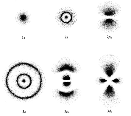
The end and the beginning

The hydrogenic atom really is about the most complicated system for which an analytical solution is possible. For anything more complicated, we can only use numerical methods to get approximate values for the energies of the system. In the application of Quantum Mechanics to chemistry, we build up our approximate wavefunctions for molecules from combinations of these hydrogenic wavefunctions. So, in this module we have brought you only as far as the threshold of chemistry: we have stopped just after introducing the orbital shapes that are all familiar to you from the first chapters of your general chemistry textbooks! But now you should have a better idea of where they come from. If you want to pursue Quantum Chemistry further, you should enrol in PHYS 301 for third year.

Summary

This module provides an introduction to the formal theory of quantum mechanics and illustrates its use with applications to some simple systems. The following lists the new concepts that have been introduced. Ensure that you are familiar with all the points listed and revise appropriate sections where necessary.

• The origins of quantum mechanics; failures of classical physics, wave-particle duality.
• The dynamics of microscopic systems; Schrödinger equation, Born interpretation of the wavefunction.
• Quantum mechanical principles; information in a wavefunction, the uncertainty principle.
• Translational motion; particle in a box, motion in two or more dimensions, tunneling.
• Vibrational motion; energy levels and wavefunctions.
• Rotational motion; rotation in three dimensions; energy levels and wavefunctions.
• The structure and spectra of hydrogenic atoms; atomic orbitals and their energies; visualisation of atomic orbitals.